Pricing Theory
The carbon pricing matrix could turn a systemic crisis into a systemic opportunity.
— Dr. Delton Chen (Founder)
Contents
Introduction
Carbon Pricing Matrix
1. Video 1
2. Video 2
Technical Background
1. Carrots and Sticks: Maximising Cooperation
2. Costs and Risks: Car Driver Example
3. Costs and Risks: The Trade-Off Problem
4. Costs and Risks: The Climate Crisis
5. Systemic Externality: Thinking Outside the Box
6. Complementary Social Principles
7. Pricing Risk with Rewards
Footnotes [a][b][c][d][e]
Record of edits between 14-17 February 2024:
Numerous edits were made to update the theory and improve this webpage, including
a) ‘Optimal growth’ was replaced with ‘balanced growth in carbon’.
b) The text describing costs and risks was improved for clarity.
c) The notion of a ‘systemic externality’ was introduced as a major new feature of the theory.
d) A section for complementary social principles was added.
e) The market failure is renamed a ‘thermodynamic market failure’ in footnote c.
Introduction
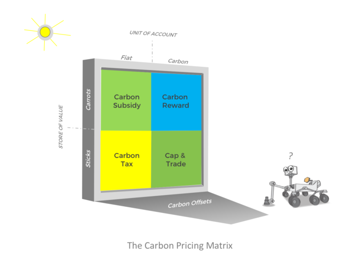
The carbon pricing matrix is framed by ‘carrot’ and ‘stick’ incentives. It explicitly defines four major carbon pricing options: carbon taxes, cap-and-trade, carbon subsidies, and the proposed carbon reward. All four are recommended here for responding to the climate crisis.
The Technical Background to the carbon pricing matrix is presented below. This background includes a hypothesis that ‘carrot and stick’ incentives can be used to maximise social cooperation for managing the anthropogenic carbon cycle. It is proposed here that the carbon pricing matrix — given its focus on cooperation and providing scalable finance — could turn a systemic crisis into a systemic opportunity.
Important is that the carbon pricing matrix is used to support and advance a new economic development pathway called balanced economic growth in carbon, which is defined on the homepage. Balanced growth in carbon has two major objectives that are managed in a trade-off: (1) social efficiency in production and consumption, and (2) a safely managed carbon cycle. A biophysical interpretation of balanced growth in carbon will eventually be presented on this website in a separate section, called Biophysical Analysis (refer the menu).
In addition to the four policies shown in the matrix, there may also exist other market tools called carbon credits. These are often used for offsetting emissions. Carbon offsetting can also interface with voluntary initiatives, including with private initiatives to adopt an internal carbon cap, usually framed as a net-zero pledge. Private actors may also adopt internal carbon taxes, called shadow pricing. These market tools are not examined here for reasons of brevity, however a carbon pricing classification table (not shown) was developed from the carbon pricing matrix to help explain all of these pricing options.
The various possible hybrid policies, such as fee-and-dividend and fee-rebates, are not discussed here because they are only hybrids of the major policies shown in Figure 1.
The non-market governmental policies, which are not covered in this review, include planning laws, emissions standards, regulations, ecocide laws, political commitments, and Green New Deals, etc. Also not shown in Figure 1 are the initiatives of non-state actors, such as climate bonds, philanthropy, ESG reporting, impact investing, etc. These initiatives of non-state actors could have a beneficial impact on the carbon cycle, but they are not discussed here because their impact is relatively small.
Carbon Pricing Matrix
Video 1. Short introduction to the carbon pricing matrix (7 minutes)
Footnote to Video 1: see Carbon Currency for a description of the four functions of money.
Each of the four quadrants of the carbon pricing matrix represents a unique market policy. Each market policy employs an instrument. Each instrument has a unit of account — either ‘fiat’ or ‘carbon’ units — represented by the two columns of the matrix. Each instrument has a store of value — either as a ‘carrot’ or as a ‘stick’— represented by the two rows of the matrix.
The (1) unit of account and the (2) store of value are two of the four major functions of money. The other functions of money are (3) medium of exchange and (4) social agreement. These four functions are relevant to the analysis of market policies because these policies are concerned with influencing prices. However, market policies employ only three of the four functions of money because the medium of exchange function is already provided by national fiat currencies. In other words, the medium of exchange function is not associated with the carbon reward policy or any other policy in the carbon pricing matrix.
In summary, the carbon pricing matrix is a relational diagram for just three functions: (i) unit of account, (ii) store of value, and (iii) social agreement. The social agreements that associate with the four market policies in the matrix need to be defined using theory that is external to the matrix, as explained below. The main focus of the following discussion is to define the four social agreements of the matrix. Note that the carbon reward policy does not appear in the mainstream economics literature, and so the aim here is to derive its social agreement via deductive reasoning.
The social agreement for the carbon tax — a stick — is the the objective of correcting (i.e. internalising) the social cost that is generated by anthropogenic carbon emissions. The social agreement for the carbon reward — a carrot — is defined here as the objective of managing the risks that associate with the carbon cycle, including carbon emissions, carbon removals, and the various stores of carbon including the whole biosphere. For these market policies to deliver on their objectives, these policies must have the capacity to improve social and political cooperation otherwise these policies will not be fully implemented. It is claimed here that a combination of carrots and sticks is actually needed to achieve the required cooperation (see Carrots and Sticks: Maximising Cooperation below).
A 17 minute YouTube video is provided (see Video 2) to introduce the key economic concepts and theories that are used to justify the four policies of the carbon pricing matrix, including the carbon tax, cap-and-trade, carbon subsidy, and the newly proposed carbon reward. Video 2 is somewhat more detailed than Video 1, and it explains why carbon offsetting is used, and how carbon offsetting relates to the carbon pricing matrix.
An explanation for why the carbon pricing matrix can/should be used to manage (a) social costs with sticks, and (b) carbon-related risks with carrots, is provided in the Technical Background, Footnotes, and the section on Biophysical Analysis.
Technical Background
1. Carrots and Sticks: Maximising Cooperation
Several scientific studies — including by Andreoni et al. (2003), Hilbe and Sigmund (2010), and Chen et al. (2014) — provide circumstantial evidence that financial rewards can improve cooperation. These studies found that cooperation amongst people involved in competitive games improves significantly when exposed to both carrot and stick incentives. This under-appreciated scientific finding is adopted as an emergent feature of the carbon pricing matrix.
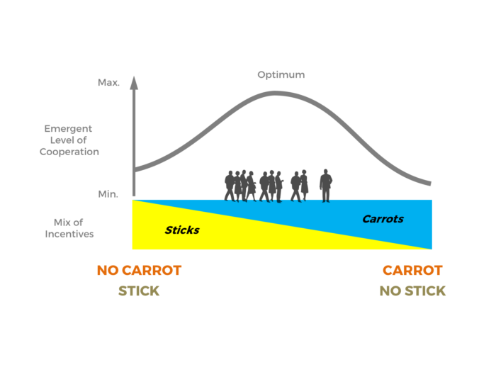
It is claimed here that cooperation for mitigating the climate crisis is currently far below optimal because the standard theory on carbon pricing is heavily biased towards taxes and cap-and-trade (i.e. sticks). A key feature of the carbon pricing matrix is that it highlights the option to balance sticks with carrots as a major new way of improving cooperation and managing the anthropogenic carbon balance.
Figure 2. Group cooperation tends to maximise when ‘carrot’ and ‘stick’ incentives are combined.
The combination of carrot and stick incentives has a “profound effect” on cooperation (Andreoni et al., 2003) and it is “…a surprisingly inexpensive and widely applicable method of promoting cooperation” (Chen et al., 2014).
The recommended ‘carrots’ are the carbon reward and the carbon subsidy—which create positive prices for mitigated carbon. The recommended ‘sticks’ are the carbon tax and cap-and-trade—which create negative prices for emitted carbon.
The carbon pricing matrix and the theory for cooperation (see Figure 2) are also based on the following three presumptions: (1) there will be strong business interest in the profit opportunities that will be created by the carbon reward, (2) there will be strong market demand for the carbon currency given that it will be managed as an investment-grade currency with significant year-on-year appreciation, and (3) there will be much greater community involvement in climate mitigation based on the financial stimulus and new job opportunities created by the carbon reward, thereby shifting public opinion in favour of strong climate mitigation even if this involves higher carbon taxes and more stringent emissions regulations.
2. Costs and Risks: Car Driver Example
The standard technical definition of risk is that it is “the effect of uncertainty on objectives” (ISO 3100). Many people simply define risk as the probability of an event multiplied by the impact of the event. The essential idea behind these definitions is that risks are unwanted events that are probabilistic in magnitude and/or their timing. Costs, on the other hand, usually refer to events that have predictable outcomes and can be planned for.
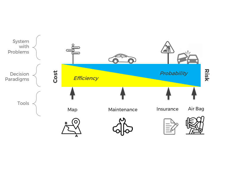
To help explain the meaning of costs and risks, some of the costs and risks of driving a car are presented in Figure 3. The yellow and blue wedges in Figure 3 are symbolic of the relative importance of the costs and the risks to the driver, respectively.
Figure 3. Responding to the costs and risks of driving a car with decisions and tools
Footnotes to Figure 3: (a) risk is the inverse of safety; and (b) the wedge diagram is based on efficiency (%) and probability (%) because these are non-dimensional values for describing problems and their solutions.
The yellow wedge is labeled “efficiency”, because choices that are made by the driver to manage costs are often made by comparing the efficiency of available options (i.e. high versus low efficiency). The blue wedge is labeled “probability”, because choices that are made for managing risks are often made by evaluating and addressing the probability of undesirable events (i.e. is the probability a concern?). The shape of the two wedges implies that all problems involve a combination of costs and risks in some proportion.
Problems and tools dominated by cost considerations are located close the left side of the wedge diagram in Figure 3; and problems and tools dominated by risk considerations are located close to the right side of the wedge diagram in Figure 3. Problems and tools that address a mix of costs and risks appear near the middle of the wedge diagram.

The driver uses two decision paradigms to manage the car as a system. One to maximise efficiency, and the other to manage probabilities.
Let’s consider an example of a cost. When the driver plans a journey from point A to point B, the most efficient route is typically the one that has the shortest distance (see Figure 3). A shorter route is usually more efficient because it requires less fuel and time. A tool that is often used to reduce these input costs is a roadmap or a GPS that displays the available routes. Given that a roadmap is a tool for managing efficiency, it is shown on the left side of the wedge diagram (see Figure 3).
Let’s consider the example of a risk. When driving on public roads, there exists a probability that the driver might collide with another vehicle. Collisions are a risk for all drivers. The driver in this example buys an air bag as physical insurance in the event of a collision. Given that the airbag is a tool for increasing the probability of surviving a car accident, it is shown on the right side of the wedge diagram (see Figure 3). The driver may also buy an insurance policy to convert the financial risk of accidents and collisions into a predictable cost (see Figure 3).
Although some tools may be useful for improving efficiency and for managing probabilities — such as a visiting a car mechanic (see Figure 3) — we should appreciate that certain tools are specialised for managing costs, by improving efficiency, and certain tools are specialised for managing risks, by influencing or responding to probabilities.
We may now describe the decision paradigms for managing costs and risks. The first decision paradigm is to improve efficiency, and the main example is to select the journeys with the highest efficiency, as follows:
1. Decision Paradigm for Efficiency: Car Driver Example
| Efficiency = Benefit of Arriving at a Destination (Output) / Cost of Driving (Input) | Example of Efficiency-Based Decision Paradigm |
The efficiency-based decision paradigm (see above) may be called cost-benefit analysis (CBA). If the inputs and outputs can be expressed in the same units, then the efficiency can be expressed as a pure percentage (%).
With regards to the management of risks, the decision paradigm is to compare the probability (%) of unwanted events with the risk appetite of the driver, as follows:
2. Decision Paradigm for Probability: Car Driver Example
| Risk mitigation is needed if the probability of a dangerous event exceeds the driver’s risk appetite | Example of Risk-Based Decision Paradigm |
3. Costs and Risks: The Trade-Off Problem
One example of a trade-off between costs and risks — in a highly controlled artificial environment — is found in the control of a spacecraft when it docks with another spacecraft. According to Vinod and Oishi (2018), this trade-off problem involves a number of key factors, including the spacecraft’s trajectory, timing, measurement errors, and fuel needs. So a spacecraft pilot, just like a car driver (refer above), has to deal with costs and risks!

If the management of climate risk is expensive, then a loss of economic efficiency may be needed in a tradeoff to reduce the climate risk.
Another example of a trade-off between costs and risks is the world’s response to the COVID-19 pandemic. The risk was a function of the probability that the disease would spread among citizens. In this example, the governments of the world responded by imposing social distancing and other measures to reduce the probability of infection, and this introduced major constraints on many business operations, and thus its reduced economic efficiency in a trade-off. The IMF reports that real global GDP contracted by 3.3% in 2020 because of the constraints placed on certain kinds of trade.
4. Costs and Risks: The Climate Crisis
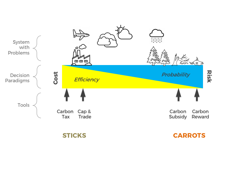
Footnotes to Figures 4 & 5: (a) risk is the inverse of safety; and (b) the wedge diagram is based on efficiency (%) and probability (%) because these are non-dimensional values for describing problems and their solutions.
The decision paradigm for costs is represented in Figures 4 & 5 by the yellow wedge and is labeled “efficiency”. It requires cost vs. benefit analysis (refer 1. Decision Paradigm for Efficiency). The decision paradigm for risks is represented by the blue wedge and is labeled “probability”. It requires a response to probabilities (refer 2. Decision Paradigm for Probability).
The decision paradigm presented as the yellow wedge in Figures 4 & 5 is applied to the maximisation of economic efficiency (i.e. for a socially efficient marketplace). This decision paradigm is essential to the standard design of the carbon tax. The way that the carbon tax is evaluated, is with the method of Arthur Pigou (1920), which is to apply cost-benefit analysis (CBA), as follows:
1. Decision Paradigm for Efficiency: Market Economy
| The social efficiency of the marketplace is improved when taxes on pollution equal the marginal damages of the pollution. | Efficiency-Based Decision Paradigm |
The decision paradigm for managing the risks associated with the anthropogenic carbon balance is symbolised by the blue wedge in Figure 4. This decision paradigm aims to compare the probability of unwanted climate change with the risk appetite of society, as follows:
2. Decision Paradigm for Probability: Market Economy
| Risk mitigation is needed if the probability of dangerous systemic change exceeds the risk appetite of society | Risk-Based Decision Paradigm |
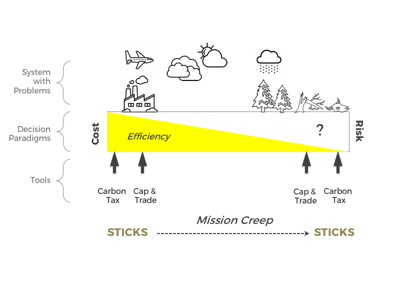
Figure 5 illustrates the status quo on carbon pricing, where the carbon tax is proposed for two objectives: (1) improving the social efficiency of the marketplace (refer 1. Decision Paradigm for Efficiency), and (2) addressing the 2015 Paris Climate Agreement which was formulated to limit the risks and impacts of dangerous climate change (refer 2. Decision Paradigm for Probability). We know that the Paris Agreement is focused on risk management because the following statement appears in Article 2:
❝Holding the increase in the global average temperature to well below 2°C above pre-industrial levels and pursuing efforts to limit the temperature increase to 1.5°C above pre-industrial levels, recognizing that this would significantly reduce the risks and impacts of climate change; ❞
The key difference between Figures 4 & 5 is that the risk-based decision paradigm (i.e. 2. Decision Paradigm for Probability) is overlooked in the standard theory for carbon pricing. The result is ‘mission creep’ for the carbon tax, cap-and-trade and other ‘sticks’. This mission creep is the result of proposing that taxes can/should be used to manage two criteria: (1) costs and (2) risks. There are two problems with this approach. First, the optimisation of costs and risks may be in conflict, requiring a trade-off between the two. Second, taxes are not suited to the task of managing systemic risks because they do not solicit enough social and political cooperation.
The key difference between Figures 4 and 5 is further discussed in Footnote [b] in relation to the work of two leading economists, William Nordhaus and Nicholas Stern, and also in relation to multivariate optimisation.
5. Systemic Externality: Thinking Outside the Box
With negative externalities being in the spotlight, we need to remind ourselves that there can exist other kinds of externality, including positive externalities. A positive externality is a spillover benefit that is enjoyed by a third-party who does not pay for the benefit. What creates a positive externality is called a merit good. A merit good is a good or service that provides significant benefits for people who do not pay. Examples are education and healthcare, because they often produce spillover benefits for society as a whole.
In this theory for the carbon reward policy and the carbon pricing matrix (refer Figure 1), we need to think beyond the concepts of negative and positive externalities, as defined by Arthur Pigou in 1920, because these externalities only relate to the choices of market actors and this is why they are referred to as social costs and benefits, respectively. Pigou’s theory is currently the ‘standard theory’ in economics but our attention needs to widen to take a broader perspective. We need to consider the possibility that market failures can be created and worsened by economic systems. If we entertain this new idea, then we may need to define a new type of externality to understand the market failure in carbon.
Let’s consider the possibility that the market failure in carbon is partly the result of the system of fiat money creation, which is a debt-based system of money creation called ‘bank credit’. If this debt-based system is a driving force for encouraging continuous profits, higher profits, and economic growth, then it appears reasonable to conclude that the market failure in carbon is worsened by debt accumulation because this amplifies the profit motive resulting in unsustainable economic activity such as fossil fuel extraction and dirty consumption. We need a new term to describe this systemic impact of the economy on carbon emissions. We call this impact a ‘systemic externality‘. BY definition, the systemic externality is the hidden cost that the economic system plays in perpetuating and worsening the market failure in carbon. Given that economic systems are metaphorically speaking the ‘rules of the game’, it is posited here that the cost of correcting the systemic externality should not be imposed on market actors because market actors are not responsible for making the rules.
Now, let’s consider more carefully the cost of managing the systemic risk associated with the carbon cycle. First, let’s consider the example of buying car insurance to manage the risk of a car accident (refer Figure 3). In this example we may agree that the risk is limited by buying an insurance policy with a predictable cost. Similarly, if we attempt to manage the systemic risk using the carbon reward policy, the cost of funding the policy should be predictable. Furthermore, the cost of funding the carbon reward policy should not be imposed on market actors because market actors are not responsible for the design of the economy and so they are not responsible for the systemic externality. In effect, the government is responsible for the economic system and so the government is the metaphorical ‘driver’ when comparing with the car driver example (refer Figure 3). So, to correct the market failure in carbon, the cost of funding the carbon reward policy can be channeled into currency markets, with the help of monetary policy, to avoid imposing any additional costs on market actors. This process of correcting the market failure with the help of the carbon reward policy may be described as ‘monetising’ the systemic externality.
This approach to correcting the market failure (i.e. internalising the negative externality with the carbon tax, and monetising the systemic externality with the carbon reward) completes the carbon pricing matrix in terms of the social agreements that correspond to the four major policies of the matrix (see Figure 1). The omission of the systemic externality in standard market theory is considered here to be a critical blind spot in neoclassical economics. Why indeed do most economists focus on the negative externality and the carbon tax, while ignoring the role of the economic system? The answer appears to be that the polluter pays principle is a relatively simple and intuitive principle to understand, and it also appeals to the neoclassical vision of improving efficiency. The systemic externality, on the other hand, is relatively complex and unorthodox because it proposes that risk management requires a new kind of financial ‘carrot’ — the carbon reward — and a bold new social principle based on the notion of preventative insurance, as explained below.
6. Complementary Social Principles
The policies appearing in the carbon pricing matrix (Figure 1) need to be morally justified. The carbon tax and other sticks are linked to costs (refer 1. Decision Paradigm for Efficiency) and they are morally justified with the polluter pays principle, as follows:
1. Social Principle for Pollution
| The ‘polluter pays principle’ states that the party that produces the pollution should bear the costs of prevention and rehabilitation if society or the environment are impacted. | Social Principle for Addressing Social Costs |
However, the polluter pays principle has some limitations. First, it assumes that the actions of polluters are self-motivated when it is often the case that producers and consumers have limited choices because they are somewhat like ‘cogs in a wheel’, where the wheel is metaphorical for an economy that has a growth bias and a rising appetite for profits and energy. Second, pollution taxes alone are far from ideal for addressing systemic risks (refer 2. Decision Paradigm for Probability) because taxes do not attract enough social and political cooperation. These conceptual limitations are resolved with the use of carbon rewards for managing the systemic risk (refer Figures 4 & 5). The following social principle, called the preventative insurance principle, is provided as the moral justification for applying the carbon reward policy:
2. Social Principle for Mitigation
| The ‘preventative insurance principle’ states that the management of a systemic risk should be guaranteed by transferring the cost away from all stakeholders via the monetisation of the mitigation cost. |
Social Principle for Addressing Systemic Risks |
Here we introduce the concept of preventative insurance because the required climate mitigation services are analogous to preventative health care when trying to avoid an incurable disease. Unlike regular healthcare, the direct cost of the preventative insurance should be transferred away from market actors and other stakeholders, and this is to avoid political conflict over the sharing of costs. The recommended approach is to use the monetary policy described in the section on Currency Demand. This monetary policy will transfer the mitigation cost away from stakeholders thus improving cooperation and increasing the effectiveness of the reward policy. Finally, to correct the entire market failure in terms of costs and risks, a combination of carrot and stick carbon pricing should be applied as implied with the carbon pricing matrix (refer Figure 1).
7. Pricing Risk with Rewards
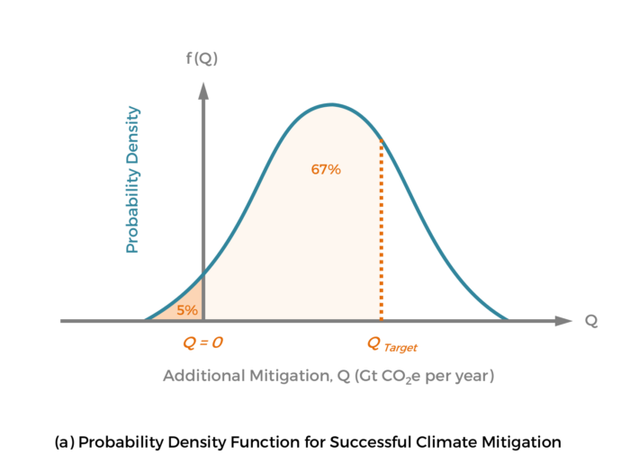
With regards to the Paris Agreement, the objective is to limit global warming to a maximum of 1.5 to 2.0°C relative to the pre-industrial baseline, but without specifying the probability of success. In this policy the probability of success is described with the PDF like the one shown in Figure 6a. This PDF shows a hypothetical mitigation challenge for remaining below 2°C of global warming with a 67% chance of success (i.e. a 33% chance of failure).
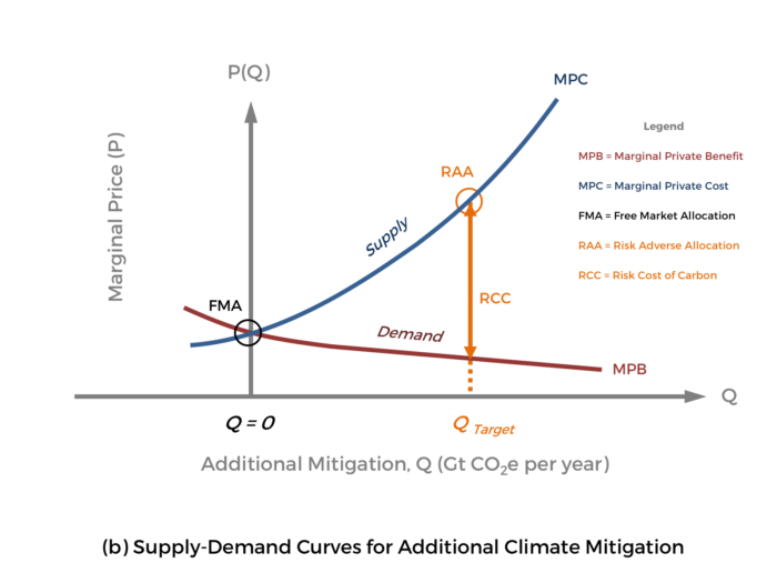
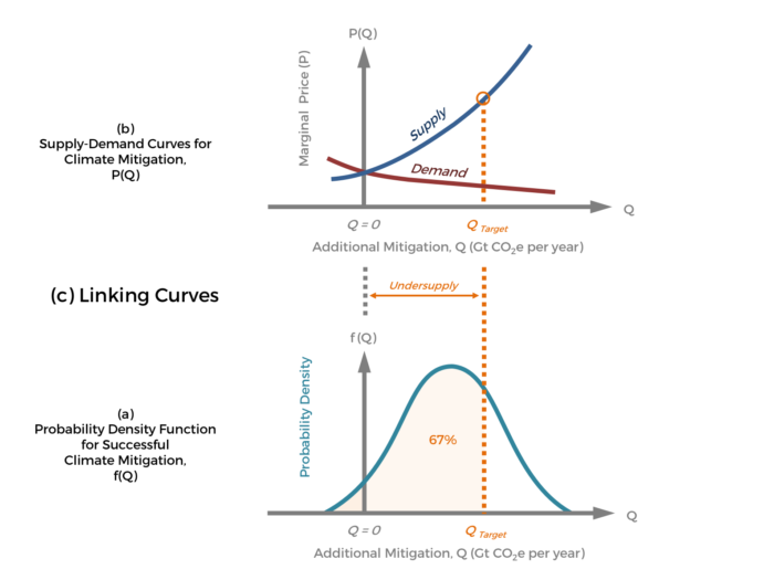
Figure 6. Hypothetical example of using a carbon reward to incentivise markets to remain below 2°C of global warming with 67% chance of success: (a) probability density function for successful climate mitigation, f(Q); (b) supply-demand curves for additional climate mitigation, P(Q); and (c) linking f(Q) with P(Q).
The carbon reward policy will price various kinds of mitigation — including atmospheric carbon removal and emission reductions for all strategically important industries. Important, is that the additional mitigation, Q(t), is comprised of two parts — (1) carbon reductions, and (2) carbon removal — but the price P(t) is only calibrated to the carbon removal as a long-term global price signal. The target amount of carbon removal will be the minimum safe level of carbon removal given the likely trajectory of residual emissions over the long-term. In other words, the carbon reward policy will establish an explicit global price for a minimum safe level of carbon removal, and this price will be estimated a priori.
The carbon reductions (avoided emissions) are managed with flexible pricing and bespoke formulas that can address the many nuances of each particular sector and industry. This flexible pricing is based on notional mass avoided, whereas the explicit pricing for carbon removal is based on actual mass removed. For reasons of brevity, the policy approach for flexible pricing is not explained here, and these details are provided in other presentations on this website. The minimum safe level of carbon removal is compared with the best estimate of the supply-demand curve for carbon removal in order to evaluate the carbon reward price (P) as illustrated in Figure 6b. The supply-demand curve should include the administrative cost of the policy as well as the removal cost.
Three system types — societal, built and Earth — should be taken into consideration when assessing the PDFs and the supply-demand curves for additional mitigation (see Table 1). Built systems include the full spectrum of technologies and methods that can be used to reduce carbon emissions and remove carbon from the ambient atmosphere. It is important to note that carbon rewards do not pick technology ‘winners and losers’ because the rewards are only provided for successful outcomes. In other words, market participants are expected to carry the financial risk of their projects.
Table 1. Systems that have an impact on the probability of mitigating climate change.
1. Societal Systems
-
- Financial
- Political
- Institutional
- Legal
- Educational
- Media
- Family Planning
2. Built Systems
-
- Energy Production
- Food Production
- Buildings & Cities
- Land & Sea Use
- Transport
- Materials Production
- Carbon Dioxide Removal (CDR)
3. Earth Systems
-
- Atmosphere (Air)
- Hydrosphere (Water)
- Cryosphere (Ice)
- Biosphere (Ecosystems)
- Pedosphere (Soil & Rocks)
Footnote to Table 1: The probability density function (PDF) for successful climate mitigation is a function of the rate of additional climate mitigation (Q) by mass. The PDF will be influenced by human interference with the Earth’s albedo, however such influences should be treated as independent variables and managed outside of the carbon pricing matrix. Solar radiation management (SRM), if it is needed, will likely require new top-down not-for-profit policies and global governance (refer Biophysical Analysis).
The ideal reward price, P(t), is called the risk cost of carbon (RCC). The RCC is the counterpart to the social cost of carbon (SCC) when evaluating the ideal carbon tax. A distinctive feature of the RCC is that the supply-demand curves (refer Figure 6) do not include marginal social costs or benefits. They only show marginal private costs and benefits. Social costs and benefits are simply ignored because they do not actually exist. This is because the ‘systemic externality’ is monetised, and the monetisation process is the responsibility of regulatory institutions.
A distinctive feature of the RCC and the carbon reward is that its evaluation does not involve any social time discounting, and this is because the RCC is framed by a rolling 100-year planning horizon. The RCC is only time discounted in terms of the total length of the rolling planning horizon. The 100-year planning horizon is based on critical path analysis, in which it is presumed that events during the next 100 years will disproportionally impact events during the following millennia. The critical path analysis takes into account the irreversibility of damages (e.g. species extinction and ecosystem collapse) and the uncertainty of tipping points. It also presumes that significant technological advances and re-organisation can take place over a 100-year period.
Updated 9 January 2022
Footnotes
Stern and his colleagues at the High Level Commission on Carbon Pricing recommend a carbon tax that targets the Paris Agreement. The framing of their assessment is ambiguous with regards to the decision paradigm (see this report and the right side of Figure 5). On the one hand, Stern et al’s decision paradigm is based on addressing the Paris Agreement (i.e. 2. Decision Paradigm for Probability). On the other hand, it appears that Stern et al have assumed that the market theory of Arthur Pigou (1920) should give the same result (i.e. 1. Decision Paradigm for Efficiency). It is claimed here that this ambiguity is the result of ‘mission creep’ because a socially efficient market does not necessarily correspond to goals of the Paris Agreement. Moreover, it is claimed here that the carbon tax is inherently inappropriate for managing climate-related risks because it does not solicit sufficient cooperation from market participants and it has other limitations.
By comparing Figures 4 and 5, we can see that there is an alternative explanation for the discrepancy between the advice of Nordhaus and Stern et al. Although the damage function in Nordhaus’s analysis could be overly optimistic, the point of most importance is the current interpretation of “carrot and stick” carbon pricing, as depicted in Figure 4. In this revised interpretation, the resolution is the carbon pricing matrix with the second decision paradigm and the carbon reward for responding to the systemic risks of climate change.
Nordhaus and Stern et al have only utilised one formal theory for making and enforcing decisions. This theory is based on Arthur Pigou’s (1920) theory for the maximisation of market efficiency (i.e. for the welfare of society) with the re-pricing of private production to account for externalities (i.e. invoking 1. Decision Paradigm for Efficiency). The signing of the Paris Climate Agreement in 2016 was a milestone for risk management (i.e. invoking 2. Decision Paradigm for Probability). The Paris Agreement stands in contrast to the theory of Arthur Pigou (1920) because it ignores market efficiency for the purpose of managing risk.
It is claimed here that the climate crisis should be understood as a trivariate optimisation problem, based on the presumption of three degrees-of-freedom. If the Earth’s energy balance were stable, then the market failure in carbon might be understood as a bivariate optimisation problem, based on carrot and stick carbon pricing. Carrots and sticks are identified here as being two of the three required controllers, with the third controller relating to the Earth’s albedo, which can change significantly over timescales of centuries or decades. Hence, the proposed policy resolution is to take control of the carbon balance using two explicit prices on carbon, namely with sticks (including with taxes on emitted carbon) and carrots (including with rewards for mitigated carbon), and to address the albedo problem with a separate international policy that is effective for managing the Earth’s albedo.
Given that warming of the Earth’s climate system is prone to positive feedbacks — including changes in surface albedo, cloud albedo, and possible climate tipping points — it is likely that solar radiation management (SRM) technologies will be needed, and this is consistent with the notion of the three-dimensional phase space (refer Footnote [e]). If the Earth’s albedo needs to be managed, then it becomes apparent that the survivability of global civilisation is a trivariate optimisation problem based on three global variables: (1) the social efficiency of producing goods and services, (1) the probability of achieving a relatively safe carbon balance for climate stability and socio-ecological regeneration, and (3) the average albedo of the Earth.
Note that the three key variables — (1) efficiency (%), (2) probability (%) and (3) albedo (%) — are non-dimensional and are expressed as percentages. Note also, that the term ‘efficiency’ is referring to the ‘social’ efficiency of markets, and this social efficiency is likely to be strongly correlated to the energy efficiency of the means of production. It is proposed here that these three variables constitute the three-dimensional phase-space of the civilisation-Earth-climate continuum and can be used to define the conditions that are necessary for the survivability of civilisation as a self-organising system. The phase-space concept originated in the discipline of physics, and more specifically in classical thermodynamics. The three-dimensional phase space that is proposed here (i.e. based on efficiency, probability and albedo) does not appear in the literature because it is a newly proposed phase-space and is specific to complex living systems.
A theory that supports the three dimensional phase-space for civilisation (and the thermodynamic market failure) is introduced in the section termed biophysical analysis. The biophysical analysis is focused on describing the economy and living organisms as biophysical systems. The analysis links the behaviour of these living systems to the laws of thermodynamics and associated concepts, however the complete theory is not presented on this website for reasons of brevity.
If the hypothesis for a thermodynamic market failure (and the phase space) holds true, then the neoclassical framework for market externalities and carbon pricing should be revised accordingly.

